Deciding Join Order in Database Systems
The database system is one of the major components in a bunch of software projects. In particular, a widely used operation on database is join operation. For example, suppose we have two separate data stores for employee and department information in a company. How do we know the employees who work under a department located in California? In general, when we need to combine two data sources to obtain our desired results, a join operation between them is necessary, denoting their consolidation into a structured whole.
Here we will introduce a typical cost-based model to optimize join orders in database systems.
Definition of Join in the Context of Relational Databases
To manage the complexity of this article, let’s introduce the concept of join in an intuitive context of relational databases (RDB).
What is RDB?
In the first place, relational databases are based on the theory of relational algebra (from which comes the name). In relational algebra, we organize data in relations, which consist of schemes and tuples. The scheme of a relation defines what kind of data it could hold, including several attributes and their corresponding types and domains for each. A tuple holds a row of values that satisfy the requirements defined by the scheme, and there can be multiple unordered tuples in a relation.
For instance, assume the relation called employee is structured as
| e_id | name | d_id |
|---|---|---|
| 20794 | Alice | 5 |
| 68691 | Bob | 11 |
where the first row in the above table represents attribute names, and following rows are actual tuples.
Another relation department can be similarly represented as
| d_id | name | location |
|---|---|---|
| 5 | Accounting | California |
| 11 | Sales | New York |
| 17 | Engineering | California |
These relations are, of course, extremely simplified ones from real word examples. The point is to represent data in the form of such tables/relations, and a complete relational database is a collection of multiple relations possibly with additional information.
What is Join?
Let us get back to the original problem. To select qualified employees, we certainly need to combine the information from both relations. But how should we combine them in a meaningful way?
Cartesian product
Before answering it, we introduce a common operation in math called Cartesian product. Say there are $m$ x-coordinates and $n$ y-coordinates, from which we want to get an ordered pair $(x, y)$. Each x-coordinate can be combined with every y-coordinate, and vice versa. For example, if we select x-coordinate from a set $\{-1, 1\}$ and y-coordinate from $\{1, 2\}$, then it results in $\{(-1, 1), (-1, 2), (1, 1), (1, 2)\}$ whose cardinality is $2\times2=4$. Generally a Cartesian product would generate $mn$ elements.
From Cartesian product to join
Sometimes not all such combinations in a Cartesian product are meaningful. As to our example of employee and department above, if we compute the Cartesian product of tuples from both relations, pairs containing Engineering department would be meaningless since no one in employee really works in it.
Therefore, we have to filter out unnecessary results from a primitive Cartesian product operation. But what should be the criteria?
Observe that both relations have the same column name. Should we pick those resulting tuple pairs that share the same names? Probably not. It makes no sense to compare the name of a department to a person. A more intuitive option is d_id (denoting Department ID) — and we only keep the pairs whose d_id from employee matches that from department.
We call such conditional Cartesian products as join operations.
Physical Implementation
Relations
Recall that relations are conceptually tables with
- Attribute definitions
- Actual tuples
Information that describes what data are stored in a relation is called metadata, which is commonly held in a special relation in a database system. Whenever needed, the metadata can be read from this relation and used to retrieve actual data.
As we’ve seen in the example, data tuples are stored in rows, each position corresponding to an attribute. Thus it’s natural to imitate the logical model and store actual data row by row. Fortunately, in many cases data in the same relation are highly homogeneous, for which we can expect to store them in a regular manner. For data types like integers and dates, fixed-length storage (which is easy to implement and maintain) is enough in many cases.
However, a significant counterexample is variable-length strings, where additional information about the length of each row record is demanded. We do not go deep into detailed techniques here, but the implementation still focused on efficiently storing rows on disks.
Join Operations
Assume the two relations employee and department as above. Since we know rows are the basic units for data storage, it seems trivial to implement Cartesian product on them now:
result = []
for e in employee:
    for d in department:
        result.append((e, d))
We adopt Python syntax for its succinctness and strong expressive power, but it should be easily readable as pseudocode.
For joins, we simply add a conditional statement, which can be logically represented in one line:
result = [(e, d) for e in employee for d in department if cond(e, d)]
A key difference between join operations in the real world and the pseudocode above is that we use in-memory data structures for both data sources and result storage, whereas it would be barely possible to keep them in main memory even for a moderately large database due to the large number of tuples. Therefore, it’s inevitable to take account of disk operations to seek and save data.
Because data on disks are both read and written in blocks, a modified strategy would be
for e_block in employee:
    for d_block in department:
        write_to_disk(generate_joined_pairs(e_block, d_block, cond))
where function generate_joined_pairs() performs similarly as in-memory join implementation.
There are many other join implementations exploiting characteristics of relations and some specific classes of join conditions, which are significantly more sophisticated but much more efficient in certain cases. We omit further details here, but anyone interested can refer to the following links as examples:
Join Order Matters
Recall that disk operations take significantly more time than RAM and CPU cache. A typical hard disk drive with mechanical structure and magnetic materials for persistent information storage takes around 10 ms for a random I/O, contrasted with RAMs enjoying an average magnitude of 10-100 nm and caches ~1 nm. Also note that sequential I/O for hard disks would be much faster after an initial seek, though.
Evaluating joins on relations residing on disks is definitely expensive. In other words, it would be fruitful if we can somehow reduce its time cost. Let’s start from an analogous example.
Matrix Multiplication Order
We’re given an ordered sequence of matrices and we wish to compute the following product
\[M_1 M_2 \cdots M_n\]Suppose it’s a legal ordering and produces a well-defined product in terms of linear algebra.
From the associativity of matrix multiplication, we can pair any neighboring two matrices, compute their product and replace the original two matrices with the newly computed matrix product, without affecting the correctness of the final result. For example, if the sequence consists of $M_1 M_2 M_3$, we can compute the final product in two different ways:
- $(M_1(M_2 M_3))$
- $((M_1 M_2)M_3)$
Suppose further that we use the subroutine below to compute matrix multiplication:
def mult(A: List[List[int]], B: List[List[int]]) -> List[List[int]]:
    """Return product of matrices A and B, assuming len(A[0]) == len(B)"""
    p, q, r = len(A), len(B), len(B[0])
    C = [[0] * r for _ in range(p)]
    for i in range(p):
        for j in range(r):
            for k in range(q):
                C[i][j] += A[i][k] * B[k][j]
    return C
It’s easy to figure out the running time, $O(p \cdot q \cdot r)$. If the dimensions of matrices are $5 \times 100$, $100 \times 10$, $10 \times 20$ respectively, then the time costs of two multiplication approaches are
- $(100 \times 10 \times 20 + 5 \times 100 \times 20) = 30,000$
- $(5 \times 100 \times 10 + 5 \times 10 \times 20) = 6,000$
Notice the first approach takes 5 times as much time as the second! Unfortunately, for a sequence of $n$ matrices, there is an approximately exponential number of ways of multiplying them, which obstructs brute-force search for an optimal multiplication order.
Join Order of Relations
Now we try to formulate the problem of join order.
As we noted above, disk operations are required to obtain the Cartesian product (and conditional join) results of two relations. Assume the two relations use $b_1$ and $b_2$ blocks respectively in file system for data storage, roughly a total of $b_1 \cdot b_2 + b_1$ block transfers are needed, using the aforementioned nested-loop block join algorithm with $b_1$ denoting blocks of the outer relation. If we exchange the nested loops, it evaluates to $b_2 \cdot b_1 + b_2$, which is slightly different.
With the help of advanced join algorithms, we need far less time for many specific common join cases. Although we won’t give an exact analytical expression for their running time, we instead denote the cost of an optimal join between relations $r_i$ and $r_j$ by $c_{i,j}$ with implicit join conditions understood. In practice, the cost is often computed using pre-collected statistics and pre-configured parameters stored as metadata in the database.
Note especially that unlike matrix multiplications, joins are not only associative but also commutative, which contributes to much more flexible arrangements of join order. For example, if we wish to join three relations $r_1$, $r_2$, $r_3$, we may choose any of the join orders below with corresponding time cost followed:
- $((r_1 r_2) r_3)$, with cost $c_{1,2} + c_{\{1,2\}, 3}$
- $((r_2 r_1) r_3)$, with cost $c_{2,1} + c_{\{1,2\}, 3}$
- $(r_3 (r_1 r_2))$, with cost $c_{1,2} + c_{3, \{1,2\}}$
- $(r_3 (r_2 r_1))$, with cost $c_{2,1} + c_{3, \{1,2\}}$
- $\cdots$
where braces in the subscription of $c$ denotes a joined relation. Notice that different join orders have different costs, but the resulting relation remains unchanged.
Our goal is to decide an optimal join order with least (or nearly least) time cost. Considering the expense of disk operations, it’s well justified to pay for the decision process, because those computations are performed in memory.
Finding an Optimal Join Order
Brute-force algorithm is simple but effective in many situations. Why should we bother designing a sophisticated algorithm if brute force suffices to find an optimal join order?
Inherent Difficulty
Assume $n$ relations denoted by $r_1, r_2, \cdots, r_n$. For common database joins, $n \le 10$. Is it possible to take an exhaustive search among all possible join orders?
Denote the number of join orders among the set $S$ of $n$ relations by $\text{count}(n)$. The final join operation in the collection of relations must happen between an ordered pair of disjoint sets of relations. Equivalently, imagine that we’re placing elements into the left and right subtree of the root.
Note that such trees are full binary trees such that each internal node has exactly two children. The problem now is how many full binary trees can be constructed from $n$ distinct leaf nodes.
Observe that in a full binary tree with $n$ identical leaf nodes, there are $n-1$ internal nodes. Furthermore, if we remove the leaf nodes, the remaining internal nodes form a normal binary tree. Therefore, the number of full binary trees with $n$ identical leaf nodes equals the number of normal binary trees with $n-1$ nodes.
Let $b(n)$ denote the number of binary trees with $n$ nodes. We have
\[b(n) = \sum_{k=0}^{n-1}b(k)b(n-1-k)\]which is exactly the well-known Catalan number given by $\frac{1}{n+1}\binom{2n}{n}$.
Finally, we put missing $n$ leaf nodes to make it a full binary tree. When the leaf nodes are distinct, we have
\[\begin{aligned} \text{count}(n) &= b(n-1) \cdot n! \\ &= \frac{1}{n}\binom{2(n-1)}{n-1} \cdot n! \\ &= \frac{(2(n-1))!}{(n-1)!} \end{aligned}\]different full binary trees. When $n = 10$, $\text{count}(n) = 17,643,225,600$, which is surely unacceptable for modern commodity hardware.
Dynamic Programming
However, the problem exhibits good properties for dynamic programming: optimal substructure and overlapping subproblems.
Consider dividing the original set of relations into two non-empty sets $S’$ and $S - S’$. We can compute the optimal join order recursively by
\[OPT(S) = \begin{equation*} \begin{cases} \min_{S' \subset S \land S' \neq \emptyset} \{OPT(S') + OPT(S - S') + c_{S', S-S'}\} &\text{if card}(S) > 1, \\ 0 &\text{otherwise}. \end{cases} \end{equation*}\]Minimum selection takes $\Theta(2^{\text{card}(S)})$ time. So for each subset $S’$ of $S$ such that $\text{card}(S’) > 1$, we sum their evaluation time costs:
\[\begin{aligned} T(n) &= \sum_{k=2}^{n}\sum_{\text{card}(S')=k} \Theta(2^{\text{card}(S')}) \\ &= \Theta (\sum_{k=2}^{n} \binom{n}{k}2^k) \\ &= \Theta(3^n - 2n - 1) \\ &= \Theta(3^n) \end{aligned}\]which evaluates to $T(10) \approx 59049$ unit operations, taking drastically less time than brute-force. In addition, we can record the current minimum join cost and prune unnecessary searches to save more time.
Implementation in Python
For simplicity, we assume all joins degenerate to Cartesian products and the only available join algorithm is the general-purpose nested-loop block join.
"""
We supply a function opt_join_order() to compute both minimum join cost
and optimal join order. For example,
>>> opt_join_order([10])
(0, 10)
>>> opt_join_order([5, 5])
(30, (5, 5))
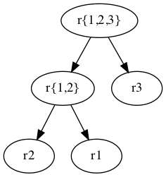
>>> opt_join_order([1, 2, 3])
(11, ((1, 2), 3))
"""
import functools
import math
from collections import Counter
from itertools import chain, combinations
from typing import (Any, Iterable, Iterator, List,
NamedTuple, Optional, Tuple, Union, cast)
JoinOrder = Union[int, Tuple]
JoinPair = Tuple['Multiset', 'Multiset']
class Multiset:
"""A logically immutable multiset based on Counter."""
def __init__(self, iterable: Iterable):
self._cnt = Counter(iterable)
def __eq__(self, other: Any) -> bool:
return self._cnt == other._cnt if isinstance(other, Multiset) else False
def __hash__(self) -> int:
return hash(frozenset(self._cnt.items()))
def __iter__(self) -> Iterator[int]:
return self._cnt.elements()
def __len__(self) -> int:
return sum(self._cnt.values())
def __sub__(self, other: Any) -> 'Multiset':
if not isinstance(other, Multiset):
raise TypeError(f'Multiset required, but {type(other)} passed.')
return Multiset(self._cnt - other._cnt)
def powerset(self) -> Iterator['Multiset']:
"""Return an iterator of non-empty proper subsets."""
return map(Multiset, chain.from_iterable(combinations(self, r)
for r in range(1, len(self))))
def opt_join_order(relations: List[int]) -> Tuple[int, JoinOrder]:
"""Return minimum join cost with an optimal join order as a nested tuple.
Parameters:
relations -- a non-empty list of positive integers denoting
the number of blocks occupied by each relation.
"""
class Result(NamedTuple):
cost: int = 0
pair: Optional[JoinPair] = None
@functools.cache
def min_join_cost(rels: Multiset) -> Result:
"""Return minimum join cost with a pair of relations whose joining
results in the optimal cost.
"""
def join_cost(outer: Multiset, inner: Multiset) -> int:
"""Return nested-loop block join cost of outer and inner relations."""
return math.prod(outer) * (math.prod(inner) + 1)
results = (Result(cost=min_join_cost(subset).cost
+ min_join_cost(rels - subset).cost
+ join_cost(subset, rels - subset),
pair=(subset, rels - subset))
for subset in rels.powerset())
return min(results, key=lambda r: r.cost, default=Result())
def reconstruct_join_order(rels: Multiset) -> JoinOrder:
"""Return the nested tuple denoting an optimal join order."""
if len(rels) == 1:
return next(iter(rels))
else:
joining_pair = cast(JoinPair, min_join_cost(rels).pair)
return tuple(map(reconstruct_join_order, joining_pair))
rels = Multiset(relations)
return min_join_cost(rels).cost, reconstruct_join_order(rels)
if __name__ == '__main__':
import doctest
doctest.testmod()
Dealing with More Relations
Though not commonly seen, there are cases in which we wish to join a large number of relations. Dynamic programming no longer satisfies our needs now, or else the time saving in actual join operations is more than offset by the cost of optimal join order computation.
In practice, many database systems simply employ a greedy strategy to decide the join order among a larger number of relations aside from regular dynamic programming approach. It is worthy of note that PostgreSQL implements a heuristic genetic algorithm to find a possible global optimum in a large search space.